7 Getting Your Data Right
7.1 This Chapter
- we will discuss how to get your data into a proper shape:
- how to extract data from printed sources;
- how to “tidy” your data, that is to say to how prepare it for the use with the tidyverse approach; how to normalize your data, which is also a part of tidying your data;
- how to model your data, which is about getting more from your data during analyses;
- then, we will look into the PUA dataset and our main task will be to create an improved version of it that is most suitable for different forms of analyses with the tidyverse approach.
7.2 1. Getting your own data
7.2.1 Ways of obtaining data
- Reusing already produced data
- One may require to mold data into a more fitting structure .
- Creating one’s own dataset
- Digitizing data from printed and/or hand-written sources
7.2.2 Major formats
- Relational databases or Tables/Spreadsheets (tabular data)?
- Tabular format: tables; spreadsheets; CSV/TSV files;
- Unique identifiers:
- tables with different data can be connected via unique identifiers
- Note: A relational database (rDB) is a collection of interconnected tables. Tables in an rDB are connected with each other via unique identifiers which are usually automatically created by the database itself when new data is added.
- In the PUA data, we have
idPersonajein the mainpersonajetable, and then in all thepersonaje_xtables, which connect individuals and their relevant descriptions. For example, we can connectpersonajeandlugarviapersonaje_lugarand analyze the geography of people from the database.
- In the PUA data, we have
- One can maintain interconnected tables without creating a rDB with a Linked Open Data approach (LOD); or, better Linked Local Data approach. The main idea is that we create unique identifiers to all entities that we use—then we can use these identifiers to expand our data either manually, semi-automatically, or automatically.
7.2.3 Ways of obtaining data
- Reusing already produced data
- One may require to mold data into a more fitting structure.
- Creating one’s own dataset
- Digitizing data from printed and/or hand-written sources
7.2.4 Major formats
- Relational databases or Tables/Spreadsheets (tabular data)?
- Tabular format: tables; spreadsheets; CSV/TSV files.
- Unique identifiers:
- tables with different data can be connected via unique identifiers
- Note: A relational database (rDB) is a collection of interconnected tables. Tables in an rDB are connected with each other via unique identifiers which are usually automatically created by the database itself when new data is added.
- One can maintain interconnected tables without creating a rDB: Open Linked Data; (Local Linked Data: you simply connect datasets that you create and have on your computer;)
- Example: Table of the growth of cities. One table includes information on population over time; Another table includes coordinates of the cities from the dataset. It is more efficient and practical (reducing error rate from typos) to work on these tables separately, and connect them via unique identifiers of cities which are used in both tables.
7.2.4.1 Note on the CSV/TSV format
CSV stands for comma-separated values; TSV — for tab-separated values.
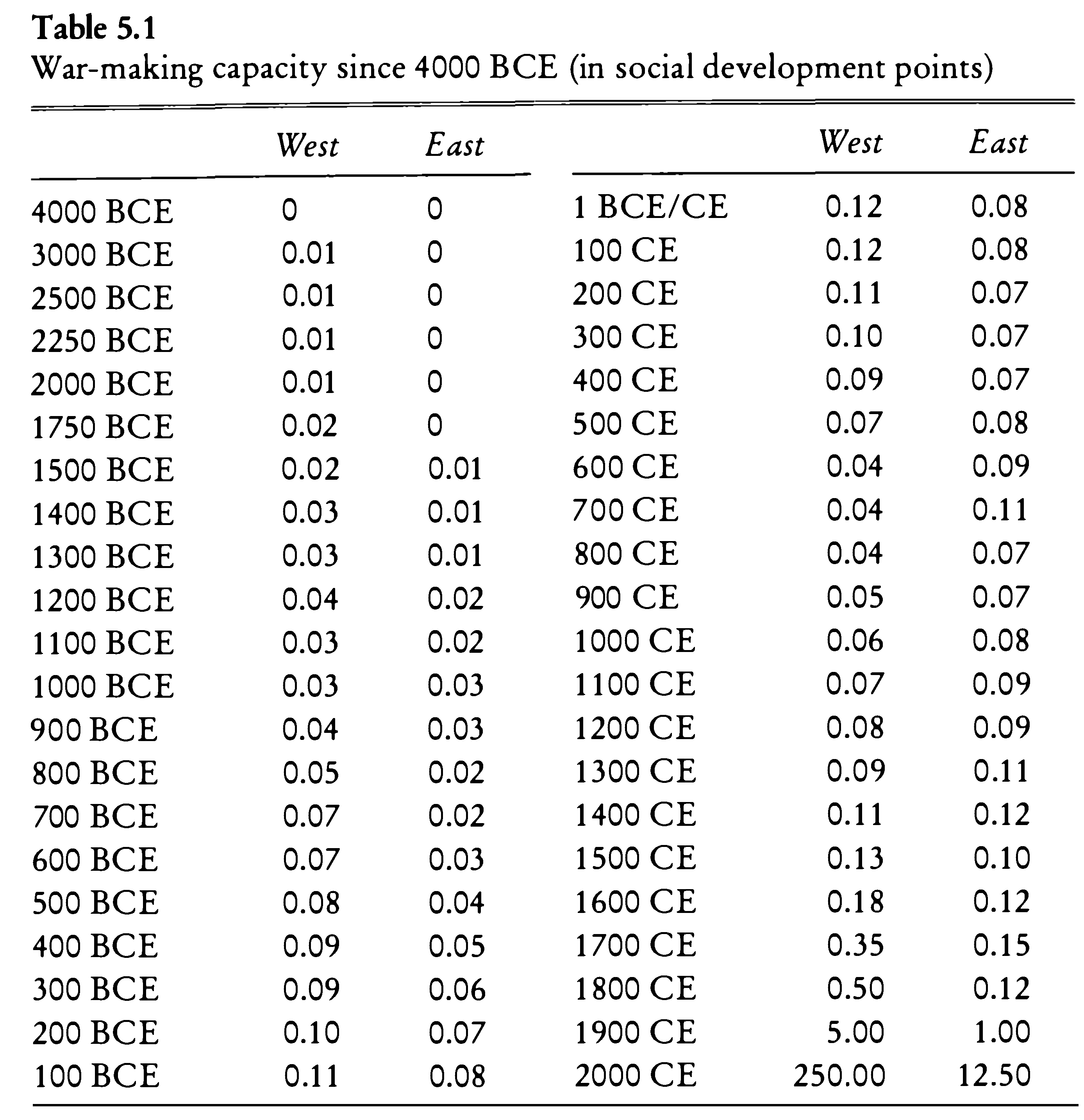
Below is an examples of a CSV format. Here, the first line is the header, which provides the names of columns; each line is a row, while columns are separated with , commas.
DATE,West,East,DATE,West,East
4000 BCE,0,0,1 BCE/CE,0.12,0.08
3000 BCE,0.01,0,100 CE,0.12,0.08
2500 BCE,0.01,0,200 CE,0.11,0.07
2250 BCE,0.01,0,300 CE,0.10,0.07
2000 BCE,0.01,0,400 CE,0.09,0.07
1750 BCE,0.02,0,500 CE,0.07,0.08
1500 BCE,0.02,0.01,600 CE,0.04,0.09
1400 BCE,0.03,0.01,700 CE,0.04,0.11
1300 BCE,0.03,0.01,800 CE,0.04,0.07
1200 BCE,0.04,0.02,900 CE,0.05,0.07
1100 BCE,0.03,0.02,1000 CE,0.06,0.08
1000 BCE,0.03,0.03,1100 CE,0.07,0.09
900 BCE,0.04,0.03,1200 CE,0.08,0.09
800 BCE,0.05,0.02,1300 CE,0.09,0.11
700 BCE,0.07,0.02,1400 CE,0.11,0.12
600 BCE,0.07,0.03,1500 CE,0.13,0.10
500 BCE,0.08,0.04,1600 CE,0.18,0.12
400 BCE,0.09,0.05,1700 CE,0.35,0.15
300 BCE,0.09,0.06,1800 CE,0.50,0.12
200 BCE,0.10,0.07,1900 CE,5.00,1.00
100 BCE,0.11,0.08,2000 CE,250.00,12.50
Example for pasting into Excel: the very last value will be misinterpreted. (The example is: War-making capacity since 4000 BCE (in social development points), from: Morris, Ian. 2013. The Measure of Civilization: How Social Development Decides the Fate of Nations. Princeton: Princeton University Press.)
TSV is a better option than a CSV, since TAB characters (\t) are very unlikely to appear in values.
Neither TSV not CSV are good for preserving new line characters (\n)—or, in other words, text split into multiple lines/paragraphs. As a workaround, one can convert \n into some unlikely-to-occur character combination (for example, ;;;), which would be easy to restore into \n later, if necessary.
7.3 2. Tidying Data
7.3.1 Basic principles of organizing data: Tidy Data
Tidy data is a concept in data organization and management introduced by statistician Hadley Wickham. It refers to a specific structure of organizing data sets in a way that is easy to analyze and manipulate, typically in the context of data science and statistical analysis. Tidy data adheres to the following principles:
- Each variable is in its own column: This means that every column represents a single variable or feature, making it easy to understand and analyze the data.
- Each observation is in its own row: This ensures that each row represents a unique observation or data point, allowing for simple indexing and filtering of the data.
- Each value is in its own cell: By having individual values in separate cells, the data is clearly organized and easy to manipulate or analyze using various data processing tools and techniques.
The need to use tidy data arises for several reasons:
- Simplified analysis: Tidy data makes it easier to perform exploratory data analysis, as the consistent organization allows for the straightforward application of various data manipulation and statistical analysis techniques.
- Improved readability: The structure of tidy data is intuitive and easy to understand, even for those with limited experience in data analysis. This makes the data more accessible for interpretation, collaboration, and communication.
- Code efficiency: With a consistent data structure, analysts can write more efficient and reusable code, as the same functions can be applied across various tidy data sets. For example, you can create an analytical routine in R that requires your data to be in a specific format—after that you can take any relevant data, convert it into the needed structure and simply reuse your R routine.
- Reduced errors: Tidy data reduces the potential for errors in data analysis by minimizing the need for manual data reshaping and transformation, which can introduce errors or inconsistencies.
- Better data quality: Tidy data encourages good data management practices by promoting the organization of data in a clear and consistent manner, making it easier to identify and address data quality issues.
In summary, adopting tidy data principles helps streamline data analysis processes, enhance collaboration, and improve the overall quality and accuracy of data-driven insights.
The original paper: Wickham, Hadley. 2014. “Tidy Data.” Journal of Statistical Software 59 (10). https://doi.org/10.18637/jss.v059.i10. (The article in open access)
7.3.2 Clean Data / Tidy Data: additional explanations
- Column names and row names are easy to use and informative. In general, it is a good practice to avoid
spacesand special characters.- Good example:
western_cities - Alternative good example:
WesternCities - Bad example:
Western Cities (only the largest)
- Good example:
- Obvious mistakes in the data have been removed:
- Date format:
YYYY-MM-DDis the most reliable format. Any thoughts why? - There should be no empty
cells: * If you have them, it might be that your data is not organized properly. * If your data is organized properly,NAmust be used as an explicit indication that data point is not available. - Each cell must contain only one piece of data.
- Variable values must be internally consistent
- Be consistent in coding your values:
Mandmanare different values computationally, but may have the same meaning in the dataset; - Keep track of your categories, i.e., keep a separate document where all codes used in the data set are explained.
- Be consistent in coding your values:
- Preserve original values:
- If you are working with a historical dataset, it will most likely be inconsistent.
- For example, distances between cities are given in different formats: days of travel, miles, farsaḫs/parasangs, etc.).
- Instead of replacing original values, it is better to create an additional column, where this information will be homogenized according to some principle.
- Keeping original data will allow to homogenize data in multiple ways (example: day of travel).
- Clearly differentiate between the original and modified/modeled values.
- The use of suffixes can be convenient:
Distance_OrigvsDistance_Modified.
- The use of suffixes can be convenient:
- If you are working with a historical dataset, it will most likely be inconsistent.
- Most of editing operations should be performed in software other than R; any spreadsheet program will work, unless it cannot export into CSV/TSV format.
- Keep in mind that if you prepare your data in an Excel-like program, rich formatting (like manual highlights, bolds, and italics) is not data and it will be lost, when you export your data into CSV/TSV format.
- Keep in mind also that programs like Excel tend to overdo it. For example, they may try to guess the format of a cell and do something with your data that you do not want. (Example for pasting into Excel)
- Note: It might be useful, however, to use rule-based highlighting in order, for example, to identify bad values that need to be fixed.
- Back up your data! In order to avoid any data loss, you need to have a good strategy to preserve your data periodically.
- http://github.com is a great place for this, plus it allows to work collaboratively.
- Google spreadsheets is a decent alternative as it allows multiple people to work on the same dataset, but it lacks version control and detailed tracking of changes.
Example for pasting into Excel: the very last value will be misinterpreted. (The example is: War-making capacity since 4000 BCE (in social development points), from: Morris, Ian. 2013. The Measure of Civilization: How Social Development Decides the Fate of Nations. Princeton: Princeton University Press.)
DATE,West,East,DATE,West,East
4000 BCE,0,0,1 BCE/CE,0.12,0.08
3000 BCE,0.01,0,100 CE,0.12,0.08
2500 BCE,0.01,0,200 CE,0.11,0.07
2250 BCE,0.01,0,300 CE,0.10,0.07
2000 BCE,0.01,0,400 CE,0.09,0.07
1750 BCE,0.02,0,500 CE,0.07,0.08
1500 BCE,0.02,0.01,600 CE,0.04,0.09
1400 BCE,0.03,0.01,700 CE,0.04,0.11
1300 BCE,0.03,0.01,800 CE,0.04,0.07
1200 BCE,0.04,0.02,900 CE,0.05,0.07
1100 BCE,0.03,0.02,1000 CE,0.06,0.08
1000 BCE,0.03,0.03,1100 CE,0.07,0.09
900 BCE,0.04,0.03,1200 CE,0.08,0.09
800 BCE,0.05,0.02,1300 CE,0.09,0.11
700 BCE,0.07,0.02,1400 CE,0.11,0.12
600 BCE,0.07,0.03,1500 CE,0.13,0.10
500 BCE,0.08,0.04,1600 CE,0.18,0.12
400 BCE,0.09,0.05,1700 CE,0.35,0.15
300 BCE,0.09,0.06,1800 CE,0.50,0.12
200 BCE,0.10,0.07,1900 CE,5.00,1.00
100 BCE,0.11,0.08,2000 CE,250.00,12.50
7.3.3 Discussion: “A Bulliet Dataset”
 |
|---|
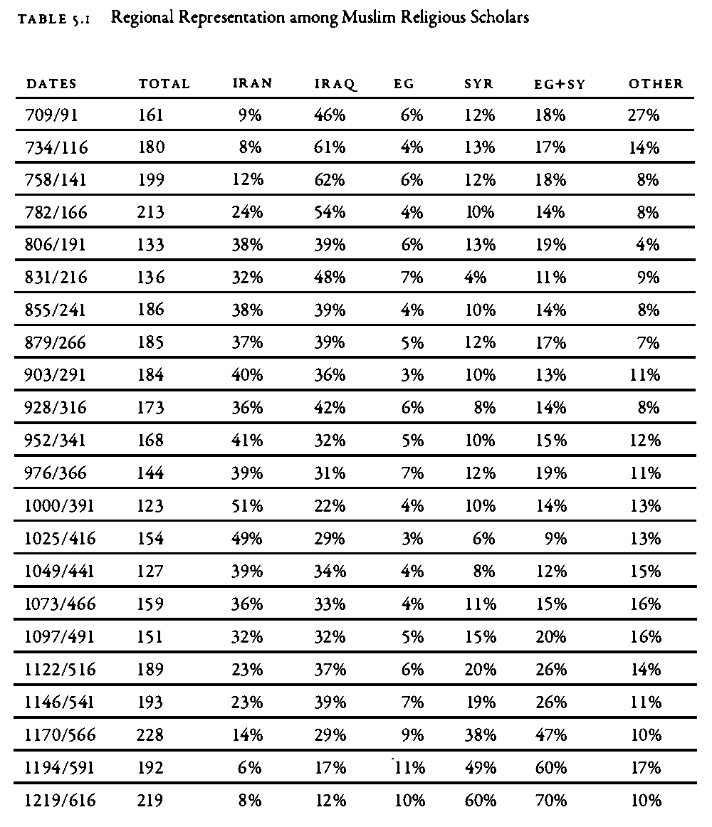
| Dataset: The dataset shows chrono-geographical distribution of Islamic scholars, according to one of the medieval biographical sources. Source: Bulliet, Richard W. 2009. Cotton, Climate, and Camels in Early Islamic Iran: A Moment in World History. New York: Columbia University Press. P. 139 |
- This data is formatted for presentation in a book; for data analysis this data needs to be converted into tidy format.
- What should be corrected? Think of how the data should look so that we could analyze it?
7.4 3. Modeling Data
7.4.1 Categorization as a Way of modeling data
“[Modeling is] a continual process of coming to know by manipulating representations.”
Willard McCarty, “Modeling: A Study in Words and Meanings,” in Susan Schreibman, Ray Siemens, and John Unsworth, A New Companion to Digital Humanities, 2nd ed. (Chichester, UK, 2016), http://www.digitalhumanities.org/companion/.
One of the most common way of modeling data in historical research—joining items into broader categories. Categorization is important because it allows to group items with low frequencies into items with higher frequencies, and through those discern patterns and trends. Additionally, alternative categorizations allow one to test different perspectives on historical data.
The overall process is rather simple in terms of technological implementation, but is quite complex in terms of subject knowledge and specialized expertise which is required to make well-informed decisions.
- For example, let’s say we have the following categories: baker, blacksmith, coppersmith, confectioner, and goldsmith.
- These can be categorized as occupations;
- Additionally, blacksmith, coppersmith, and goldsmith can also be categorized as ‘metal industry’, while baker and confectioner, can be categorized as ‘food industry’;
- Yet even more, one might want to introduce additional categories, such as luxury production to include items like goldsmith and confectioner; and regular production for items like baker, blacksmith, coppersmith.
- Such categorizations can be created in two different ways, with each having its advantages:
- first, one can create them as additional columns. This approach will allow to always have the original—or alternative—classifications at hand, which is helpful for re-thinking classifications and creating alternative ones where items will be reclassified differently, based on a different set of assumptions about your subject.
- second, these can be created in separate files, which might be easier as one does not have to stare at existing classifications and therefore will be less influenced by them in making classification decisions.
- Additionally, one can use some pre-existing classifications that have already been created in academic literature. These most likely need to be digitized and converted into properly formatted data, as we discussed in the previous lesson.
7.4.2 Normalization
This is a rather simple, yet important procedure, which is, on the technical side, very similar to what was described above. In essence, the main goal of normalization is to remove insignificant differences that may hinder analysis.
- Most common examples would be:
- bringing information to the same format (e.g., dates, names, etc.)
- unifying spelling differences
It is a safe practice to preserve the initial data, creating normalized data in separate columns (or tables)
7.4.3 Note: Proxies, Features, Abstractions
These are the terms that refer to the same idea. The notion of proxies is used in data visualization, that of features—in computer science; that of abstractions—in the humanities (see, for example, Franco Moretti’s Graph, Maps, Trees).
The main idea behind these terms is that some simple features of an object can act as proxies to some complex phenomena. For example, we can use individuals who are described as “jurists” as a proxy for the development of Islamic law. This way we use onomastic information as a proxy to the social history of Islamic law.
While proxies are selected from what is available—usually not much, especially when it comes to historical data—as a way to approach something more complex. It may also be argued that abstractions are often arrived to from the opposite direction: we start with an object which is available in its complexity—in the case of PUA, the starting point is biographies written in natural language (Arabic). The PUA researchers then reduced the complexity of biographies in natural language to a more manageable form which—we expect—would represent specific aspects of the initial complex object. From this perspective, the PUA database itself is an abstraction of biographies of Andalusians.
Most commonly (and automatically) abstractions are used with texts in natural languages. For example, in stylometry texts are reduced to frequency lists of most frequent features, which are expected to represent an authorial fingerprint. Using these frequency lists we can—with accuracy up to 99%—identify authors of particular texts. The complexity of texts can be reduced in a number of ways: into a list of lemmas (e.g., for topic modeling analysis), frequency lists (e.g., for document distance comparison, such as, for example, stylometry), keyword values (e.g., for identifying texts on a similar topic, using, for example, the TF-IDF method), syntactic structures, ngrams, etc. As you get to practice and experiment more, you will start coming up with your own ways of creating abstractions depending on your current research questions.
7.5 Appendix: OCR with R
As we discussed above, sometimes one may really need to OCR text from PDFs and images. One can do that with R in the following manner.
The following libraries will be necessary.
This code we can use to OCR individual PNG files.
text <- tesseract::ocr(pathToPNGfile, engine = tesseract("eng"))
readr::write_lines(text, str_replace(pathToPNGfile, ".png", ".txt"))
This code can be used to process entire PDFs:
imagesToProcess <- pdftools::pdf_convert(pathToPDFfile, dpi = 600)
text <- tesseract::ocr(imagesToProcess, engine = tesseract("eng"))
readr::write_lines(text, str_replace(pathToPDFfile, ".pdf", ".txt"))
NB: I had issues running pdftools on Mac. Make sure that you install additional required tools for it. For more details, see: https://github.com/ropensci/pdftools.
More details on how to use Tesseract with R you can find here: https://cran.r-project.org/web/packages/tesseract/vignettes/intro.html