7 Text Analysis I: Basics
7.1 Goals
- basic text analysis concepts;
- word frequencies and word clouds;
- word distribution plots;
- kwic: keywords-in-context
7.2 Preliminaries
7.2.1 Data
We will use the following text files in this worksheet. Please download them and keep them close to your worksheet. Since some of the files are quite large, you want to download them before loading them into R:
In order to make loading these files a little bit easier, you can paste the path to where you placed these files into an isolated variable and then reuse it as follows (in other words, make sure that your pathToFiles is the path on your local machine):
pathToFiles = "./files/data/"

d1862 <- read.delim(paste0(pathToFiles, "dispatch_1862.tsv"), encoding="UTF-8", header=TRUE, quote="")
sw1 <- scan(paste0(pathToFiles, "sw1.md"), what="character", sep="\n")
The first file is articles from “The Daily Dispatch” for the year 1862. The newspaper was published in Richmond, VA — the capital of the Confederate States (the South) during the American Civil War (1861-1865). The second file is a script of the first episode of Star Wars :).
7.2.2 Libraries
The following are the libraries that we will need for this section. Install those that you do not have yet.
#install.packages("tidyverse", "readr", "stringr")
#install.packages("tidytext", "wordcloud", "RColorBrewer"", "quanteda", "readtext")

# General ones
library(tidyverse)
library(readr)
library("RColorBrewer")

# Text Analysis Specific
library(stringr)
library(tidytext)
library(wordcloud)
library(quanteda)
library(readtext)
7.2.3 Functions in R (a refresher)
Functions are groups of related statements that perform a specific task, which help breaking a program into smaller and modular chunks. As programs grow larger and larger, functions make them more organized and manageable. Functions help avoiding repetition and makes code reusable.
Most programming languages, R including, come with a lot of pre-defined—or built-in—functions. Essentially, all statements that take arguments in parentheses are functions. For instance, in the code chunk above, read.delim() is a function that takes as its arguments: 1) filename (or, path to a file); 2) encoding; 3) specifies that the file has a header; and 4) not using " as a special character. We can also write our own functions, which take care of sets of operations thet we tend to repeat again and again.
Later, take a look at this video by one of the key R developers, and check this tutorial.
7.2.3.1 Simple Function Example: Hypothenuse
(From Wikipedia) In geometry, a hypotenuse is the longest side of a right-angled triangle, the side opposite the right angle. The length of the hypotenuse of a right triangle can be found using the Pythagorean theorem, which states that the square of the length of the hypotenuse equals the sum of the squares of the lengths of the other two sides (catheti). For example, if one of the other sides has a length of 3 (when squared, 9) and the other has a length of 4 (when squared, 16), then their squares add up to 25. The length of the hypotenuse is the square root of 25, that is, 5.
Let’s write a function that takes lengths of catheti as arguments and returns the length of hypothenuse:
hypothenuse <- function(cathetus1, cathetus2) {
  hypothenuse<- sqrt(cathetus1*cathetus1+cathetus2*cathetus2)
  print(paste("In the triangle with catheti of length",
              cathetus1, "and", cathetus2,
              ", the length of hypothenuse is",
              hypothenuse))
  return(hypothenuse)
}
Let’s try a simple example:
hypothenuse(3,4)## [1] "In the triangle with catheti of length 3 and 4 , the length of hypothenuse is 5"## [1] 5Let’s try a crazy example:
hypothenuse(390,456)## [1] "In the triangle with catheti of length 390 and 456 , the length of hypothenuse is 600.029999250037"## [1] 600.03###$ More complex one: Cleaning Text
Let’s say we want to clean up a text so that it is easier to analyze it: 1) convert everithing to lower case; 2) remove all non-alphanumeric characters; and 3) make sure that there are no multiple spaces:
clean_up_text = function(x) {
  x %>%
    str_to_lower %>% # make text lower case
    str_replace_all("[^[:alnum:]]", " ") %>% # remove non-alphanumeric symbols
    str_replace_all("\\s+", " ") # collapse multiple spaces
}
Let’s test it now:
text = "This is a sentence with punctuation, which mentions Hamburg, a city in Germany."
clean_up_text(text)
## [1] "this is a sentence with punctuation which mentions hamburg a city in germany "7.3 Texts and Text Analysis
We can think of text analysis as means of extracting meaningful information from structured and unstructured texts. As historians, we often do that by reading texts and collecting relevant information by taking notes, writing index cards, summarizing texts, juxtaposing one texts against another, comparing texts, looking into how specific words and terms are used, etc. Doing text analysis computationally we do lots of similar things: we extract information of specific kind, we compare texts, we look for similarities, we look differences, etc.
While there are similarities between traditional text analysis, there are of course, also significant differences. One of them is procedural: in computational reading we must explicitly perform every step of our analyses. For example, when we read a sentence, we, sort of, automatically identify the meaningful words — subject, verb, object, etc.; we identify keywords; we parse every word, identifying what part of speech it is, what is its lemma (i.e. its dictionary form, etc.). By doing these steps we re-construct the meaning of the text that we read — but we do most of these steps almost unconsciously, especially if a text is written in our native tongues. In computational analysis, these steps must be performed explicitly (in the order of growing complexity):
- Tokenization: what we see as a text made of words, the computer sees as a continuous string of characters (white spaces, punctuation and the like are characters). We need to break such strings into discreet objects that computer can understand construe as words.
- Lemmatization: reduces the variety of forms of the same words to their dictionary forms. Another, somewhat similar procedure is called
stemming, which usually means the removal of most common suffixes and endings to get to the stem (or, root) of the word. - POS (part-of-speech tagging): this is where we run some NLP tool that identifies the part of speech of each word in our text.
- Syntactic analysis: is the most complicated procedure, which is also usually performed with some NLP tool, which analyzes syntactic relationships within each sentence, identifying its subject(s), verb(s), object(s), etc.
NOTE:
- NLP: natural language processing;
- Token: you can think of token as a continuous string of letter characters, as a word as it appears in the text in its inflected forms with possible other attached elements (in Arabic we often have prepositions, articles, pronominal suffixes, which are not part of the word, but attached to it);
- Lemma: the dictionary form of the word;
- Stem: a “root” of the word;
Some examples:
#install.packages("textstem")
library(textstem)

sentence = c(
  "He tried to open one of the bigger boxes.",
  "The smaller boxes did not want to be opened.",
  "Different forms: open, opens, opened, opening, opened, opener, openers."
  )
The library textstem does lemmatization and stemming, but only for English. Tokenization can be performed with str_split() function — and you can define how you want your string to be split.
- Tokenization
str_split(sentence, "\\W+")## [[1]]
## [1] "He" "tried" "to" "open" "one" "of" "the" "bigger"
## [9] "boxes" ""
##
## [[2]]
## [1] "The" "smaller" "boxes" "did" "not" "want" "to"
## [8] "be" "opened" ""
##
## [[3]]
## [1] "Different" "forms" "open" "opens" "opened" "opening"
## [7] "opened" "opener" "openers" ""- Lemmatization
lemmatize_strings(sentence)## [1] "He try to open one of the big box."
## [2] "The small box do not want to be open."
## [3] "Different form: open, open, open, open, open, opener, opener."- Stemming
stem_strings(sentence)## [1] "He tri to open on of the bigger box."
## [2] "The smaller box did not want to be open."
## [3] "Differ form: open, open, open, open, open, open, open."Note: It is often important to ensure that all capital letters are converted into small letters or the other way around; additionally, some normalization procedures may be necessary to reduce orthographic complexities of specific languages (for example, ö > oe in German; simplification of forms of alif in Arabic, etc.).
7.4 Word Frequencies and Word Clouds
Let’s load all issues of Dispatch from 1862.
library(tidytext)

d1862 <- read.delim(paste0(pathToFiles, "dispatch_1862.tsv"), encoding="UTF-8", header=TRUE, quote="")

kable(head(d1862))| id | date | type | header | text |
|---|---|---|---|---|
| 1862-06-25_article_1 | 1862-06-25 | article | The lines. | The lines. On Monday night signal rockets were frequently seen to ascend from our exteme left, important of future events, and from preparations everywhere visible we were led to suppose that transactions of a mementous charactor would have transpired yesterday. but despite every conjecture nothing whatever occurred of importance. Sharp skirmishing is of daily occurrence on our extreme left, but the results have not yet been fully developed. Several wounded in these affairs have arrived in the city and report the enemy unwontedly pugnactous in that direction, although from every indication, we are ted to believe that their increasing appetite for slanghter will be more than fully satisfied are many hours shall have passed over us. A few prisoners were brought into our Lines yesterday and Monday, and from their reports it would seem that no preparations are yet perfected by the Federals for any ” onward to Richmond” movement. It is possible Libby’s warehouse will soon be honored by the arrival of a few hundred of the blue-coated gentry, and their greeting be far otherwise than as conquerors. From the interior of the enemy’s lines we learn from recent arrivals that the depredations of the foe have been frequent, their bearing remarkably imperious and overbearing — violent hands being laid upon every species of property, while aged inbabitants are daily subjected to harsh language and ill manners. Since Gen. Stuart’s visit to their rear the rancor and ill-breeding of Lincoln’s hirelings have been more than usually oppressive, their threats and taunts are increasing as to blackguardism, while the unprotected have no resort but patience and silent endurance. Indeed. Federal cavalry have been particularly active in and around Charles City, we hear; squads are patrolling all the country in search of rebels and the disloyal; but up to the present their anxiety and industry have been of no avail, for the mounted rebols have thus far cleverly cluded all traps and search. The movement of troops has been constant, but with what intent and purpose we have no positive idea. The men are in splendid order — all is enthusiasm, animation, preparation and impatience — there is an oppressive sense of incertitude, however-imaginings of bye-gone tardiness to be again rehearsed perhaps — yet all with one accord yearn for action, and are willing to trust the issue to sinewy arms and valiant hearts. An ominous slience reigus supreme-pickets in the timbor move thoughtfully to and fro without firing an accustomed shot; artillerists lean upon their guns and scan the landscape, indifferent to the seene. All is repose — the fields are moist and green, camp fires glisten and glow in the evening air, and the sun goes down upon the quietest day that we have ever seen at the Lines. The enemy are reported to have been extremely busy in their inhospitable swamp for several nights past, pickets imagine the noise to have arisen from the movements of divisions & c. Whenever the conflict shall begin, however, the sequel will demonstrate that the enemy have devised every means known to ingenuity, cunning, and malice to cause destruction among our columns. They will not trust as heretofore, in numbers, nor will they advance upon the open field and try the guage of battle. All will be left to trape, batteries, felled timber, and obstructed roads, and failing in these, panic will be universal among them, and the slaughter unprecedented.’Tis useless to conjecture a few hours perhaps, will reveal all. |
| 1862-06-25_article_2 | 1862-06-25 | article | Stuarts Reconnoissance. | Stuarts Reconnoissance. The successful raid of Gen. Stuart upon the rear of the Grand Army still continues to puzzle the Yankees, and they have not yet arrived at a full knowledge of the affair. The fact that something was done; that the Confederate cavalry was really within their lines; that a large amount of property was destroyed; that the United States dragoons were routed, and many of them taken prisoners, begins to break slowly upon their minds. It is still spoken of as the work of guerrilla parties, and a wholesome fear of these same parties has sprung up, and it is singular how many of them can be According to she statements of the correspondents, guerrilla bands are still hanging upon the near of the army, and they are seen in every quarter — sometimes at Hanover, on the Pacunkey, at White House, New Kent, Charles City, and other places. Something must be done to put a stop to such lawless proceedings; for according to the Yankee idea, a guerrilla band lurks behind every bush and in every patch of woodland. A more effectual scare has not been given since the war began. Although the rebel Stuart was finally routed and driven beyond the Chickahominy, the New York Herald says that it must be allowed by all to be one of the most daring acts ever known, and greatly to the credit of the rebels. The great excitement prevailing throughout the army, caused by this brilliant affair, is the general topic of conversation. It is perfectly incomprehensible. |
| 1862-06-25_article_3 | 1862-06-25 | article | The Yankees in King George. | The Yankees in King George. The depredations of the Yankees in King George and the adjoining counties still continue, and many of the citizens have suffered severely, having their crope destroyed, their cattle stolen, and servants carried off. The following extracts are from a letter written by a lady of King George county giving some facts regarding matters in that section:” When I last wrote to you we thought the Yankees were under good discipline, and that the officers would prevent maranding, but we soon found our mistake. They grow bolder and bolder every day, finding no troops here to oppose them, entirely destroying some farms, and wantonly shooting all the stock, while the influence they exerted over the servante was almost beyond endurance. – The Lieutenant-Colonel of a regiment now here, with 200 men, rode through our quarters, telling the servants they were all free, and as good as their masters; that they must not do any work he had come to fight for their freedom, and, if he could, he would give ten lives for them. He also invited them to come over to the camp, and bring fine horses with them. This discourse had the effect of making all the avallable men go off. Among them our coachman, in whom we had the greatest confidence. They took all our carriages and riding horses, & c. Learning that these were sometimes returned, mama went up to the camp herself. The Colonel was very polite, and gave her an order for the horses, which were restored, but the men we shall never see. I cannot deseribe to you the desolation of Fredericksburg. The town is entirely under the rule of negroes. They go to their masters and say they will not work without wages, and demand large sums for the least service; the Yankees exulting over their impertinences. They are grazing their horses on all the wheat fields, and taking every bushel of corn they can find. You remember the beautiful place of the Seddons. He is in the army, and they are eneamped on the place. No one can imagine what Mrs. S. has endured. I trust our faith will not waiver under any circumstances, and I would give up all for our beloved Confederacy.” |
| 1862-06-25_article_4 | 1862-06-25 | article | About McClellan. | About McClellan. The ” young Napoleon” had a narrow escape a short time ago of being captured by Stuart and his savalry. The Petersburg Express learns that our forces passed in their march an estate in New Kent county known as Hampstead, where Gen. McClellan has established his headquarters. At one point on the march the Confederates were within six hundred yards of Hampstead, and it has since been assertained that at the time they passed McClellan and Staff were all in the house at dinner. The only troops near were his usual body guard, numbering not more than 100 cavalry. Had Gen. Stuart been aware of the fact the building might have been surrounded and the Yankee General captured, to gether with his whole Staff. We have no doubt that within the next week the young Napoleon will wish he had been captured, for in that case, he might have avoided the thorough thrashing which is in store for him. In the latest news from from the North McClellan’s force is put down at 200, 000 although every one knows he has hardly half that number. A large number of his men are sick, and the health of the army is spoken of by a correspondent as decidedly bad. It has been said in a Yankee paper that their loss in the battle of the Chickahominy in killed wounded, missing, and demoralised amounts to 40, 000. We have no doubt it would take more than that number of men to make the army as effective as before the battle. |
| 1862-06-25_article_5 | 1862-06-25 | article | NO HEADER | Pleasant quarters. – A Yankee correspondent with Halleck’s army writes:” The troops suffer less from disease than from makes, wood ticks, lizzards, scorpions, and gallinippers. Inseets and reptties are thus classed; One Ezzard equals five scorpious; two scorpions equal one gaillnipper; one gallinipper equals one make; one snake, one gallinipper, two scorpions and one Ezzard equal one wood tick.” |
| 1862-06-25_article_6 | 1862-06-25 | article | Death of a brave man. | Death of a brave man. Capt. Jame B. Brower, of the Nansemond Cavelry, died at the residence of his brother in Prince George county, a few days since. He had been in command of this spirited envalry company for nearly a year, and had performed much service in the vicinity of Pertamouth and the Albemarie region of North Carolina. His very name was a terror to the Yankees and Union men in the vicinity of Edenton and Elizabeth City. He was a brave man. When his bealth failed he resigned his commond and yielded to death. Capt. Brewer leaves an interesting family at Suffolk. |
We can quickly check what types of articles are there in those issues.
d1862 %>%
  count(type, sort=T)
## type n
## 1 article 14639
## 2 orders 3972
## 3 advert 2023
## 4 ad-blank 535
## 5 death 233
## 6 married 186
## 7 died 70
## 8 poem 44
## 9 order 30
## 10 letter 27
## 11 ordered 15
## 12 entry 7
## 13 acticle 2
## 14 notice 2
## 15 role 2
## 16 runaway 2
## 17 article 1
## 18 25 1
## 19 Wanted 1
## 20 adverts 1
## 21 aritcle 1
## 22 artcle 1
## 23 articl 1
## 24 articler 1
## 25 aticle 1
## 26 death, 1
## 27 married, 1
## 28 marry 1
## 29 oders 1
## 30 oped 1
## 31 ordinal 1
## 32 printrun 1
## 33 ranaway 1
## 34 simple 1We can create subsets of articles based on their types.
death_d1862 <- d1862 %>%
  filter(type=="death" | type == "died")
Create subsets for other major types.
Describe problems with the data set and how they can be fixed.
your answer goes here…
Now, let’s tidy them up: to work with this as a tidy dataset, we need to restructure it in the one-token-per-row format, which as we saw earlier is done with the unnest_tokens() function.
test_set <- death_d1862

test_set_tidy <- test_set %>%
  mutate(item_number = cumsum(str_detect(text, regex("^", ignore_case = TRUE)))) %>%
  select(-type) %>%
  unnest_tokens(word, text) %>%
  mutate(word_number = row_number())

head(test_set_tidy)
## id date header item_number word word_number
## 1 1862-06-25_died_80 1862-06-25 Died. 1 died 1
## 2 1862-06-25_died_80 1862-06-25 Died. 1 on 2
## 3 1862-06-25_died_80 1862-06-25 Died. 1 monday 3
## 4 1862-06-25_died_80 1862-06-25 Died. 1 june 4
## 5 1862-06-25_died_80 1862-06-25 Died. 1 23d 5
## 6 1862-06-25_died_80 1862-06-25 Died. 1 of 6Stop words is an important concept. In general, this notion refers to the most frequent words/tokens which one might want to exclude from analysis. There are existing lists of stop words that you can find online, and they can work fine for testing purposes.
data("stop_words")

test_set_tidy_clean <- test_set_tidy %>%
  anti_join(stop_words, by="word")

head(test_set_tidy_clean)
## id date header item_number word word_number
## 1 1862-06-25_died_80 1862-06-25 Died. 1 died 1
## 2 1862-06-25_died_80 1862-06-25 Died. 1 monday 3
## 3 1862-06-25_died_80 1862-06-25 Died. 1 june 4
## 4 1862-06-25_died_80 1862-06-25 Died. 1 23d 5
## 5 1862-06-25_died_80 1862-06-25 Died. 1 12 7
## 6 1862-06-25_died_80 1862-06-25 Died. 1 o'clock 8For research purposes, it is highly advisable to develop your own stop word lists. The process is very simple:
- create a frequency list of your tokens/words;
- arrange them by frequencies in descending order;
- save top 2-3,000 in a tsv/csv file;
- open in any table editor;
- add a new column and tag those words that you want to exclude. For example,
1– for to exclude;0— for to keep. It is convenient to automatically fill the column with some default value (0), and then you can change only those that you want to remove (1).
You will see that some words, despite their frequency, might be worth keeping. When you are done, you can load them and use anti_join function to filter your corpus.
7.4.1 Word Frequencies
Let’s first count all the words:
test_set_tidy %>%
  count(word, sort = TRUE) %>%
  head(15)
## word n
## 1 the 9352
## 2 of 8148
## 3 and 5875
## 4 his 3390
## 5 to 3355
## 6 in 3272
## 7 a 2730
## 8 at 2388
## 9 on 2331
## 10 he 1595
## 11 her 1533
## 12 was 1211
## 13 o'clock 1102
## 14 from 1084
## 15 this 1084Now, let’s also remove the stop words:
test_set_tidy %>%
  anti_join(stop_words, by="word") %>%
  count(word, sort = TRUE) %>%
  head(15)
## word n
## 1 o'clock 1102
## 2 friends 992
## 3 residence 952
## 4 funeral 883
## 5 aged 763
## 6 attend 704
## 7 family 633
## 8 age 588
## 9 inst 585
## 10 died 573
## 11 invited 569
## 12 months 512
## 13 morning 481
## 14 son 453
## 15 death 4067.4.2 Wordclouds
Wordclouds can be an efficient way to visualize most frequent words. Unfortunately, in most cases, wordclouds are not used either correctly or efficiently. (Let’s check Google for some examples).
library(wordcloud)
library("RColorBrewer")

test_set_tidy_clean <- test_set_tidy %>%
  anti_join(stop_words, by="word") %>%
  count(word, sort=T)

set.seed(1234)
wordcloud(words=test_set_tidy_clean$word, freq=test_set_tidy_clean$n,
          min.freq = 1, rot.per = .25, random.order=FALSE, #scale=c(5,.5),
          max.words=150, colors=brewer.pal(8, "Dark2"))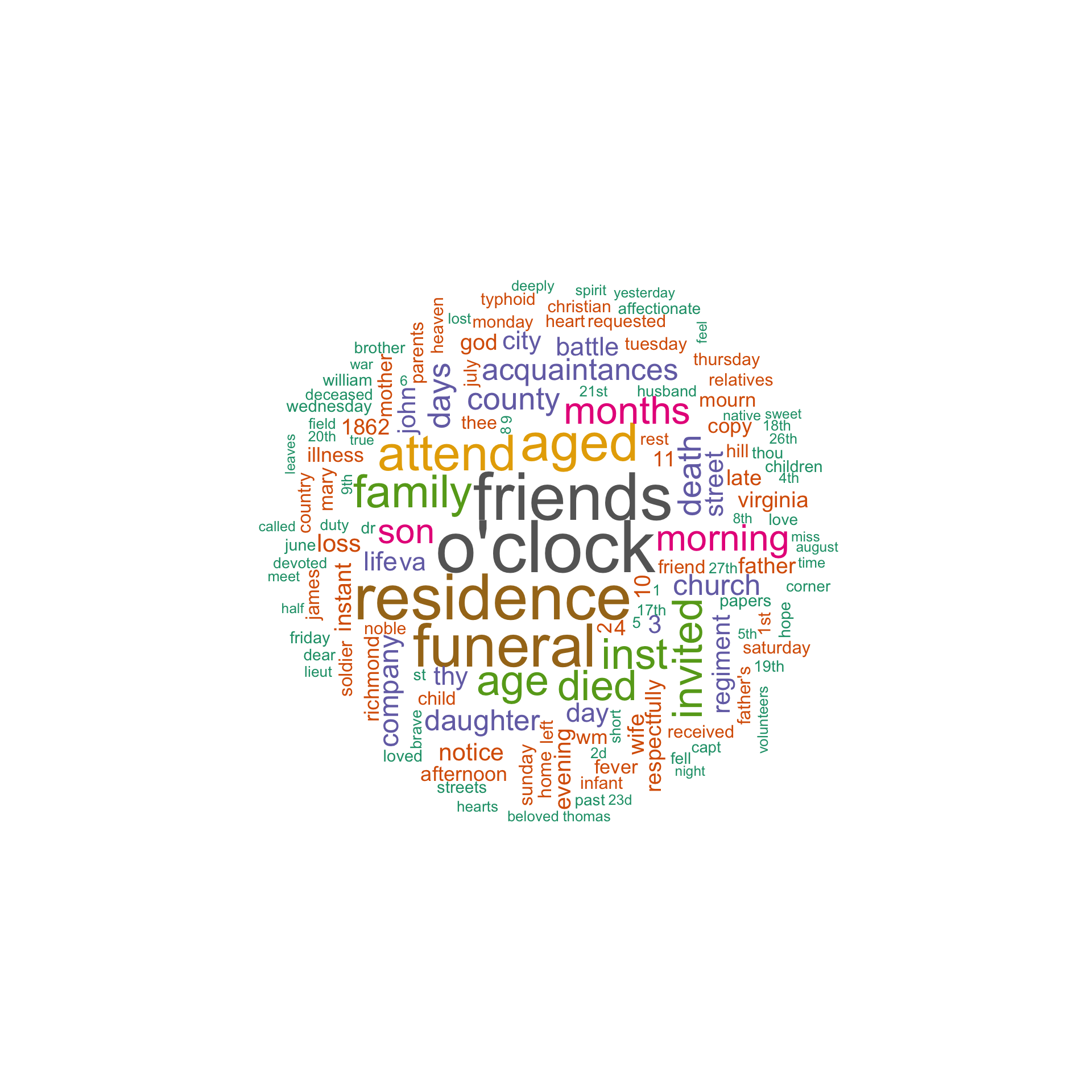
- What can we glean out form this wordcloud? Create a wordcloud for obituaries.
# your code; your response- Create a wordcloud for obituaries, but without stop words.
# your code; your response- Create a wordcloud for obituaries, but on lemmatized texts and without stop words.
# your code; your response- Summarize your observations below. What does stand out in these different versions of wordclouds? Which of the wordclouds you find more efficient? Can you think of some scenarios when a different type of wordcloud can be more efficient? Why?
you answer goes here
For more details on generating word clouds in R, see: http://www.sthda.com/english/wiki/text-mining-and-word-cloud-fundamentals-in-r-5-simple-steps-you-should-know.
7.5 Word Distribution Plots
7.5.1 Simple — a Star Wars Example
This kind of plot works better with texts rather than with newspapers. Let’s take a look at a script of Episode I:
SW_to_DF <- function(path_to_file, episode){
  sw_sentences <- scan(path_to_file, what="character", sep="\n")
  sw_sentences <- as.character(sw_sentences)
  sw_sentences <- gsub("([A-Z]) ([A-Z])", "\\1_\\2", sw_sentences)
  sw_sentences <- gsub("([A-Z])-([A-Z])", "\\1_\\2", sw_sentences)
  sw_sentences <- as.data.frame(cbind(episode, sw_sentences), stringsAsFactors=FALSE)
  colnames(sw_sentences) <- c("episode", "sentences")
  return(sw_sentences)
}

sw1_df <- SW_to_DF(paste0(pathToFiles, "sw1.md"), "sw1")

sw1_df_tidy <- sw1_df %>%
  mutate(linenumber = row_number(),
         chapter = cumsum(str_detect(sentences, regex("^#", ignore_case = TRUE))))

sw1_df_tidy <- sw1_df_tidy %>%
  unnest_tokens(word, sentences)
Try names of different characters (shmi, padme, anakin, sebulba, yoda, sith), or other terms that you know are tied to a specific part of the movie (pod, naboo, gungans, coruscant).
ourWord = "yoda"
word_occurance_vector <- which(sw1_df_tidy$word == ourWord)

plot(0, type='n', #ann=FALSE,
     xlim=c(1,length(sw1_df_tidy$word)), ylim=c(0,1),
     main=paste0("Dispersion Plot of `", ourWord, "` in SW1"),
     xlab="Movie Time", ylab=ourWord, yaxt="n")
segments(x0=word_occurance_vector, x1=word_occurance_vector, y0=0, y1=2)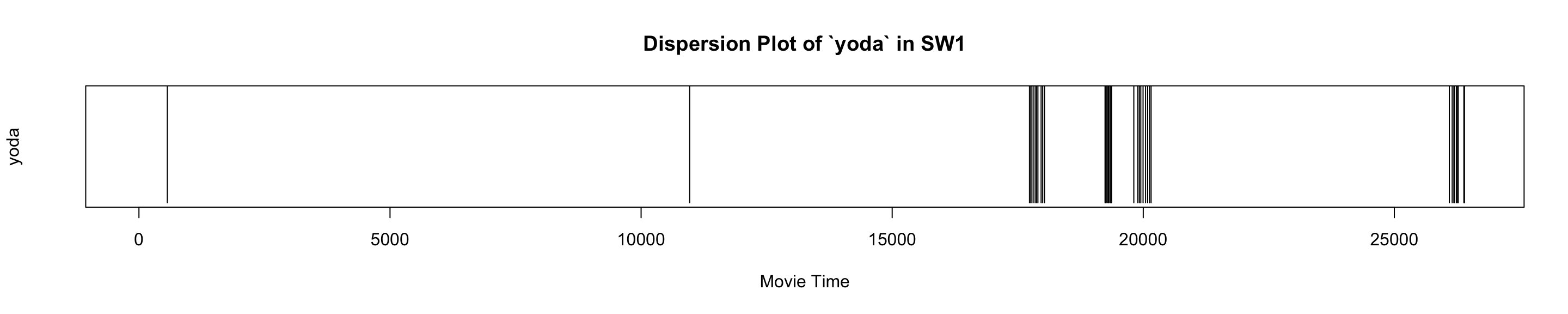
7.6 Word Distribution Plots: With Frequencies Over Time
For newspapers—and other diachronic corpora—a different approach will work better:
d1862 <- read.delim(paste0(pathToFiles, "dispatch_1862.tsv"), encoding="UTF-8", header=TRUE, quote="", stringsAsFactors = FALSE)

test_set <- d1862
test_set$date <- as.Date(test_set$date, format="%Y-%m-%d")

test_set_tidy <- test_set %>%
  mutate(item_number = cumsum(str_detect(text, regex("^", ignore_case = TRUE)))) %>%
  select(-type) %>%
  unnest_tokens(word, text) %>%
  mutate(word_number = row_number())

head(test_set_tidy)
## id date header item_number word word_number
## 1 1862-06-25_article_1 1862-06-25 The lines. 1 the 1
## 2 1862-06-25_article_1 1862-06-25 The lines. 1 lines 2
## 3 1862-06-25_article_1 1862-06-25 The lines. 1 on 3
## 4 1862-06-25_article_1 1862-06-25 The lines. 1 monday 4
## 5 1862-06-25_article_1 1862-06-25 The lines. 1 night 5
## 6 1862-06-25_article_1 1862-06-25 The lines. 1 signal 6Now, we can calculate frequencies of all words by dates:
test_set_tidy_freqDay <- test_set_tidy %>%
  anti_join(stop_words, by="word") %>%
  group_by(date) %>%
  count(word)

head(test_set_tidy_freqDay)
## # A tibble: 6 × 3
## # Groups: date [1]
## date word n
## <date> <chr> <int>
## 1 1862-01-01 000 13
## 2 1862-01-01 007 1
## 3 1862-01-01 014 1
## 4 1862-01-01 1 10
## 5 1862-01-01 10 5
## 6 1862-01-01 100 2We now can build a graph of word occurences over time. In the example below we search for manassas, which is the place where the the Second Battle of Bull Run (or, the Second Battle of Manassas) took place on August 28-30, 1862. The battle ended in Confederate victory. Our graph shows the spike of mentions of Manassas in the first days of September — right after the battle took place.
Such graphs can be used to monitor discussions of different topic in chronological perspective.
# interesting examples:
# deserters, killed,
# donelson (The Battle of Fort Donelson took place in early February of 1862),
# manassas (place of the Second Bull Run, fought in August 28–30, 1862),
# shiloh (Battle of Shiloh took place in April of 1862)

ourWord = "manassas"

test_set_tidy_word <- test_set_tidy_freqDay %>%
  filter(word==ourWord)

plot(x=test_set_tidy_word$date, y=test_set_tidy_word$n, type="l", lty=3, lwd=1,
     main=paste0("Word `", ourWord, "` over time"),
     xlab = "1862 - Dispatch coverage", ylab = "word frequency per day")
segments(x0=test_set_tidy_word$date, x1=test_set_tidy_word$date, y0=0, y1=test_set_tidy_word$n, lty=1, lwd=2)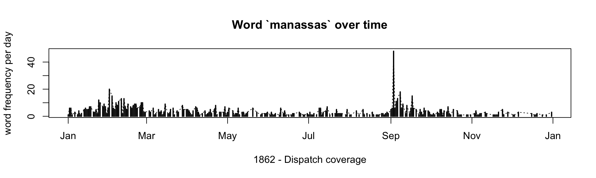
- The graph like this can be used in a different way. Try words killed and deserters. When do these words spike? Can you interpret these graphs?
your response goes here
7.7 KWIC: Keywords-in-Context
Keywords-in-context is the most common method for creating concordances — a view that that allows us to go through all instances of specific words or word forms in order to understand how they are used. The quanteda library offers a very quick and easy application of this method:
library(quanteda)
library(readtext)

dispatch1862 <- readtext(paste0(pathToFiles, "dispatch_1862.tsv"), text_field = "text", quote="")
dispatch1862corpus <- corpus(dispatch1862)
Now, we can query the created corpus object using this command: kwic(YourCorpusObject, pattern = YourSearchPattern). pattern= can also take vectors (for example, c("soldier*", "troop*")); you can also search for phrases with pattern=phrase("fort donelson"); window= defines how many words will be shown before and after the match.
kwic_test <- kwic(dispatch1862corpus, pattern = 'lincoln', window=5)## Warning: 'kwic.corpus()' is deprecated. Use 'tokens()' first.head(kwic_test)## Keyword-in-context with 6 matches.
## [dispatch_1862.tsv.57, 886] their annihilation which the infamous | Lincoln
## [dispatch_1862.tsv.58, 8] . - The Premier of | Lincoln
## [dispatch_1862.tsv.60, 1015] Saturday, two of the | Lincoln
## [dispatch_1862.tsv.129, 1447] Old Abe and Mrs. | Lincoln
## [dispatch_1862.tsv.129, 1474] kangaroo-looking person. Mrs. | Lincoln
## [dispatch_1862.tsv.129, 1530] , and wire-pullers of the | Lincoln
##
## | Government is furnishing every day
## | has declared over and over
## | gunboats came down within sight
## | , several times. Old
## | was out in her carriage
## | dynasty are violent, abusiveTo view results better, we can remove unnecessary columns:
kwic_test %>% as_tibble %>%
  select(pre, keyword, post) %>%
  head(15)
## # A tibble: 15 × 3
## pre keyword post
## <chr> <chr> <chr>
## 1 their annihilation which the infamous Lincoln Government is furnishing every…
## 2 . - The Premier of Lincoln has declared over and over
## 3 Saturday , two of the Lincoln gunboats came down within sight
## 4 Old Abe and Mrs . Lincoln , several times . Old
## 5 kangaroo-looking person . Mrs . Lincoln was out in her carriage
## 6 , and wire-pullers of the Lincoln dynasty are violent , abusive
## 7 against the boasted legions of Lincoln .
## 8 , and that Mr . Lincoln will make Gen . Banks
## 9 in the employment of the Lincoln Government had come in from
## 10 pulpit by the hirelings of Lincoln for declining to pray for
## 11 the oath of allegiance to Lincoln . It must be stipulated
## 12 off since that time . Lincoln , it will be recollected
## 13 , unexpected visit of President Lincoln , who arrived at the
## 14 the camps that Mr . Lincoln had come to have a
## 15 vociferous greeting . Mr . Lincoln rode at the right ofNB: quanteda is quite a robust library. Check this page with examples for other possible quick experiments: https://quanteda.io/articles/pkgdown/examples/plotting.html
7.8 Homework
- Read about ngrams in Chapter 4. Relationships between words: n-grams and correlations (https://www.tidytextmining.com/ngrams.html), in https://www.tidytextmining.com/.
- Using what you have learned in this chapter identify and analyze bigrams in Dispatch, 1862.
- Submit the results of your analysis as an R notebook, as usual.
- You are welcome to work in groups.
- Optional: Work through Chapter 9 of Arnold, Taylor, and Lauren Tilton. 2015. Humanities Data in R. New York, NY: Springer Science+Business Media. (on Moodle!): create a notebook with all the code discusses there and send it via email (share via DropBox or some other service, if too large).
- DataCamp Assignments.
7.9 Submitting homework
- Homework assignment must be submitted by the beginning of the next class;
- Email your homework to the instructor as attachments.
- In the subject of your email, please, add the following:
57528-LXX-HW-YourLastName-YourMatriculationNumber, whereLXXis the number of the lesson for which you submit homework;YourLastNameis your last name; andYourMatriculationNumberis your matriculation number.
- In the subject of your email, please, add the following: